Command line tutorial

This tutorial will walk you through the usage of the lib5c command-line tools.

Follow along in Google colab

You can run and modify the cells in this notebook tutorial live using Google colaboratory by clicking the link below:

To simply have all the cells run automatically, click Runtime > Run all in the colab toolbar.

Make sure lib5c is installed

Inside a fresh virtual environment, run

!pip install lib5c

Requirement already satisfied: lib5c in /mnt/c/Users/thoma/venv-doc/lib/python2.7/site-packages (0.5.3)
Requirement already satisfied: numpy>=1.10.4 in /mnt/c/Users/thoma/venv-doc/lib/python2.7/site-packages (from lib5c) (1.14.2)
Requirement already satisfied: pandas>=0.18.0 in /mnt/c/Users/thoma/venv-doc/lib/python2.7/site-packages (from lib5c) (0.22.0)
Requirement already satisfied: statsmodels>=0.6.1 in /mnt/c/Users/thoma/venv-doc/lib/python2.7/site-packages (from lib5c) (0.8.0)
Requirement already satisfied: dill>=0.2.5 in /mnt/c/Users/thoma/venv-doc/lib/python2.7/site-packages (from lib5c) (0.2.7.1)
Requirement already satisfied: luigi>=2.1.1 in /mnt/c/Users/thoma/venv-doc/lib/python2.7/site-packages (from lib5c) (2.7.3)
Requirement already satisfied: matplotlib>=1.4.3 in /mnt/c/Users/thoma/venv-doc/lib/python2.7/site-packages (from lib5c) (2.2.2)
Requirement already satisfied: python-daemon<2.2.0,>=2.1.1 in /mnt/c/Users/thoma/venv-doc/lib/python2.7/site-packages (from lib5c) (2.1.2)
Requirement already satisfied: powerlaw>=1.4.3 in /mnt/c/Users/thoma/venv-doc/lib/python2.7/site-packages (from lib5c) (1.4.3)
Requirement already satisfied: interlap>=0.2.3 in /mnt/c/Users/thoma/venv-doc/lib/python2.7/site-packages (from lib5c) (0.2.6)
Requirement already satisfied: seaborn>=0.8.0 in /mnt/c/Users/thoma/venv-doc/lib/python2.7/site-packages (from lib5c) (0.8.1)
Requirement already satisfied: decorator>=4.0.10 in /mnt/c/Users/thoma/venv-doc/lib/python2.7/site-packages (from lib5c) (4.2.1)
Requirement already satisfied: scikit-learn>=0.17.1 in /mnt/c/Users/thoma/venv-doc/lib/python2.7/site-packages (from lib5c) (0.19.1)
Requirement already satisfied: scipy>=0.16.1 in /mnt/c/Users/thoma/venv-doc/lib/python2.7/site-packages (from lib5c) (1.0.0)
Requirement already satisfied: python-dateutil in /mnt/c/Users/thoma/venv-doc/lib/python2.7/site-packages (from pandas>=0.18.0->lib5c) (2.7.2)
Requirement already satisfied: pytz>=2011k in /mnt/c/Users/thoma/venv-doc/lib/python2.7/site-packages (from pandas>=0.18.0->lib5c) (2018.3)
Requirement already satisfied: patsy in /mnt/c/Users/thoma/venv-doc/lib/python2.7/site-packages (from statsmodels>=0.6.1->lib5c) (0.5.0)
Requirement already satisfied: tornado<5,>=4.0 in /mnt/c/Users/thoma/venv-doc/lib/python2.7/site-packages (from luigi>=2.1.1->lib5c) (4.5.3)
Requirement already satisfied: pyparsing!=2.0.4,!=2.1.2,!=2.1.6,>=2.0.1 in /mnt/c/Users/thoma/venv-doc/lib/python2.7/site-packages (from matplotlib>=1.4.3->lib5c) (2.2.0)
Requirement already satisfied: backports.functools-lru-cache in /mnt/c/Users/thoma/venv-doc/lib/python2.7/site-packages (from matplotlib>=1.4.3->lib5c) (1.5)
Requirement already satisfied: subprocess32 in /mnt/c/Users/thoma/venv-doc/lib/python2.7/site-packages (from matplotlib>=1.4.3->lib5c) (3.5.3)
Requirement already satisfied: six>=1.10 in /mnt/c/Users/thoma/venv-doc/lib/python2.7/site-packages (from matplotlib>=1.4.3->lib5c) (1.11.0)
Requirement already satisfied: kiwisolver>=1.0.1 in /mnt/c/Users/thoma/venv-doc/lib/python2.7/site-packages (from matplotlib>=1.4.3->lib5c) (1.0.1)
Requirement already satisfied: cycler>=0.10 in /mnt/c/Users/thoma/venv-doc/lib/python2.7/site-packages (from matplotlib>=1.4.3->lib5c) (0.10.0)
Requirement already satisfied: setuptools in /mnt/c/Users/thoma/venv-doc/lib/python2.7/site-packages (from python-daemon<2.2.0,>=2.1.1->lib5c) (40.4.3)
Requirement already satisfied: docutils in /mnt/c/Users/thoma/venv-doc/lib/python2.7/site-packages (from python-daemon<2.2.0,>=2.1.1->lib5c) (0.14)
Requirement already satisfied: lockfile>=0.10 in /mnt/c/Users/thoma/venv-doc/lib/python2.7/site-packages (from python-daemon<2.2.0,>=2.1.1->lib5c) (0.12.2)
Requirement already satisfied: backports-abc>=0.4 in /mnt/c/Users/thoma/venv-doc/lib/python2.7/site-packages (from tornado<5,>=4.0->luigi>=2.1.1->lib5c) (0.5)
Requirement already satisfied: certifi in /mnt/c/Users/thoma/venv-doc/lib/python2.7/site-packages (from tornado<5,>=4.0->luigi>=2.1.1->lib5c) (2018.1.18)
Requirement already satisfied: singledispatch in /mnt/c/Users/thoma/venv-doc/lib/python2.7/site-packages (from tornado<5,>=4.0->luigi>=2.1.1->lib5c) (3.4.0.3)

Make a directory and get data

If you haven’t completed the pipeline tutorial yet, make a directory for the tutorial:

$ mkdir lib5c-tutorial
$ cd lib5c-tutorial

and prepare the example data in lib5c-tutorial/input as shown in the pipeline tutorial.

!mkdir input
!wget -qO- 'http://www.ncbi.nlm.nih.gov/geo/download/?acc=GSE68582&format=file&file=GSE68582%5FBED%5FES%2DNPC%2DiPS%2DLOCI%5Fmm9%2Ebed%2Egz' | gunzip -c > input/BED_ES-NPC-iPS-LOCI_mm9.bed
!wget -qO- 'http://www.ncbi.nlm.nih.gov/geo/download/?acc=GSM1974095&format=file&file=GSM1974095%5Fv65%5FRep1%2Ecounts%2Etxt%2Egz' | gunzip -c > input/v65_Rep1.counts
!wget -qO- 'http://www.ncbi.nlm.nih.gov/geo/download/?acc=GSM1974096&format=file&file=GSM1974096%5Fv65%5FRep2%2Ecounts%2Etxt%2Egz' | gunzip -c > input/v65_Rep2.counts
!wget -qO- 'http://www.ncbi.nlm.nih.gov/geo/download/?acc=GSM1974099&format=file&file=GSM1974099%5FpNPC%5FRep1%2Ecounts%2Etxt%2Egz' | gunzip -c > input/pNPC_Rep1.counts
!wget -qO- 'http://www.ncbi.nlm.nih.gov/geo/download/?acc=GSM1974100&format=file&file=GSM1974100%5FpNPC%5FRep2%2Ecounts%2Etxt%2Egz' | gunzip -c > input/pNPC_Rep2.counts
!sed -i '/Sox2\|Klf4/!d' input/BED_ES-NPC-iPS-LOCI_mm9.bed

mkdir: cannot create directory ‘input’: File exists

Note for Docker image users

If you are using lib5c from the Docker image, run:

$ docker run -it -v <full path to lib5c-tutorial>:/lib5c-tutorial creminslab/lib5c:latest
root@<container_id>:/# cd /lib5c-tutorial

and continue running all tutorial commands in this shell.

Trimming low-quality primers

We will first trim away low-quality primers by running

!lib5c trim -p input/BED_ES-NPC-iPS-LOCI_mm9.bed -t trimmed/%s.counts trimmed/primers_trimmed.bed 'input/*.counts'

creating directory trimmed

Normalization

For this tutorial, we will first use Knight-Ruiz matrix balancing to correct our data for primer effects by running

!lib5c kr trimmed/pNPC_Rep2.counts kr/pNPC_Rep2.counts

loading counts
kr balancing
writing counts
creating directory kr

lib5c kr specifies that the specific subcommand we want is kr, the subcommand for Knight-Ruiz balancing. To see all the available subcommands, you can run

!lib5c -h

                        sub-commands
    pipeline            run entire pipeline
    hic-extract         extract chunks from Hi-C data
    trim                primer and countsfile trimming
    outliers            remove high spatial outliers
    remove              remove low-count primer-primer pairs
    qnorm               quantile normalization
    express             express normalization
    kr                  knight-ruiz matrix balancing normalization
    spline              spline normalization
    iced                iced balancing normalization
    determine-bins      create binfiles from primerfiles
    bin                 bin fragment-level counts
    smooth              smooth counts
    expected            compute expected models
    variance            estimate variances from obs values and exp models
    pvalues             call pvalues for interactions
    threshold           threshold p-values
    qvalues             perform multiple testing correction
    interaction-score   convert p-values to interaction scores
    subtract            subtract countsfiles
    divide              divide countsfiles
    log                 log countsfiles
    colorscale          compute regional colorscales for comparing replicates
    plot                plot things

optional arguments:
  -h, --help            show this help message and exit
  -v, --version         show program's version number and exit

To see detailed help for the kr subcommand, you can run

!lib5c kr -h

usage: lib5c kr [-h] [-p PRIMERFILE] [-H] [-B] [-i MAX_ITERATIONS]
                [-s IMPUTATION_SIZE]
                infile outfile

positional arguments:
  infile                Input countsfile.
  outfile               Output countsfile.

optional arguments:
  -h, --help            show this help message and exit
  -p PRIMERFILE, --primerfile PRIMERFILE
                        Primer file or bin file to use. If this flag is not
                        present, a .bed file will be searched for based on the
                        locations of the input files.
  -H, --hang            If multiple input files are specified, this flag will
                        cause the terminal to hang until all input files have
                        finished processing.
  -B, --output_bias     If this flag is present, the bias vectors will be
                        written to .bias files located next to the output
                        .counts files.
  -i MAX_ITERATIONS, --max_iterations MAX_ITERATIONS
                        Maximum number of iterations. The default is 3000.
  -s IMPUTATION_SIZE, --imputation_size IMPUTATION_SIZE
                        Size of window, in units of matrix indices, to use to
                        impute nan values in the original counts matrix. Pass
                        0 to skip imputation, which is the default behavior.

The two required positional command line arguments for lib5c kr are infile (the countsfile we want to balance) and outfile (where to write the balanced countsfile).

Processing multiple input files

If we want to process a lot of countsfiles, we can use a pattern like this

!lib5c kr 'trimmed/*.counts' kr/%s.counts

lib5c kr  trimmed/pNPC_Rep1.counts 'kr/pNPC_Rep1.counts' --max_iterations '3000' --imputation_size '0'
loading counts
kr balancing
writing counts
lib5c kr  trimmed/pNPC_Rep2.counts 'kr/pNPC_Rep2.counts' --max_iterations '3000' --imputation_size '0'
loading counts
kr balancing
writing counts
lib5c kr  trimmed/v65_Rep1.counts 'kr/v65_Rep1.counts' --max_iterations '3000' --imputation_size '0'
loading counts
kr balancing
writing counts
lib5c kr  trimmed/v65_Rep2.counts 'kr/v65_Rep2.counts' --max_iterations '3000' --imputation_size '0'
loading counts
kr balancing
writing counts

Here instead of a single infile, we have put in a glob-expandable pattern that will match all the countsfiles in the input directory. We have to quote this pattern to prevent the shell from expanding it. If we are processing multiple input countsfiles, then we expect multiple countsfiles as the output. To specify this easily, we include %s in the outfile, which will be replaced with the replicate name (derived automatically from the input filenames).

If you’re running this in a cluster environment with the LSF (aka bsub) job scheduler available, you can install the bsub Python package via

$ pip install bsub

and then all the input files will be processed in parallel via bsub.

If you aren’t using the LSF job scheduler, you can still specify multiple input files, but they will be processed in series.

Plotting heatmaps

Let’s take a look at the countsfiles we just generated.

One way to visualize countsfiles is to plot heatmaps of them. To do this, we can run

!lib5c plot heatmap -p trimmed/primers_trimmed.bed --region Sox2 kr/pNPC_Rep2.counts kr/pNPC_Rep2_Sox2.png

loading counts
preparing to plot
plotting

The resulting image should look something like this

from IPython.display import Image
Image(filename='kr/pNPC_Rep2_Sox2.png', width=400)

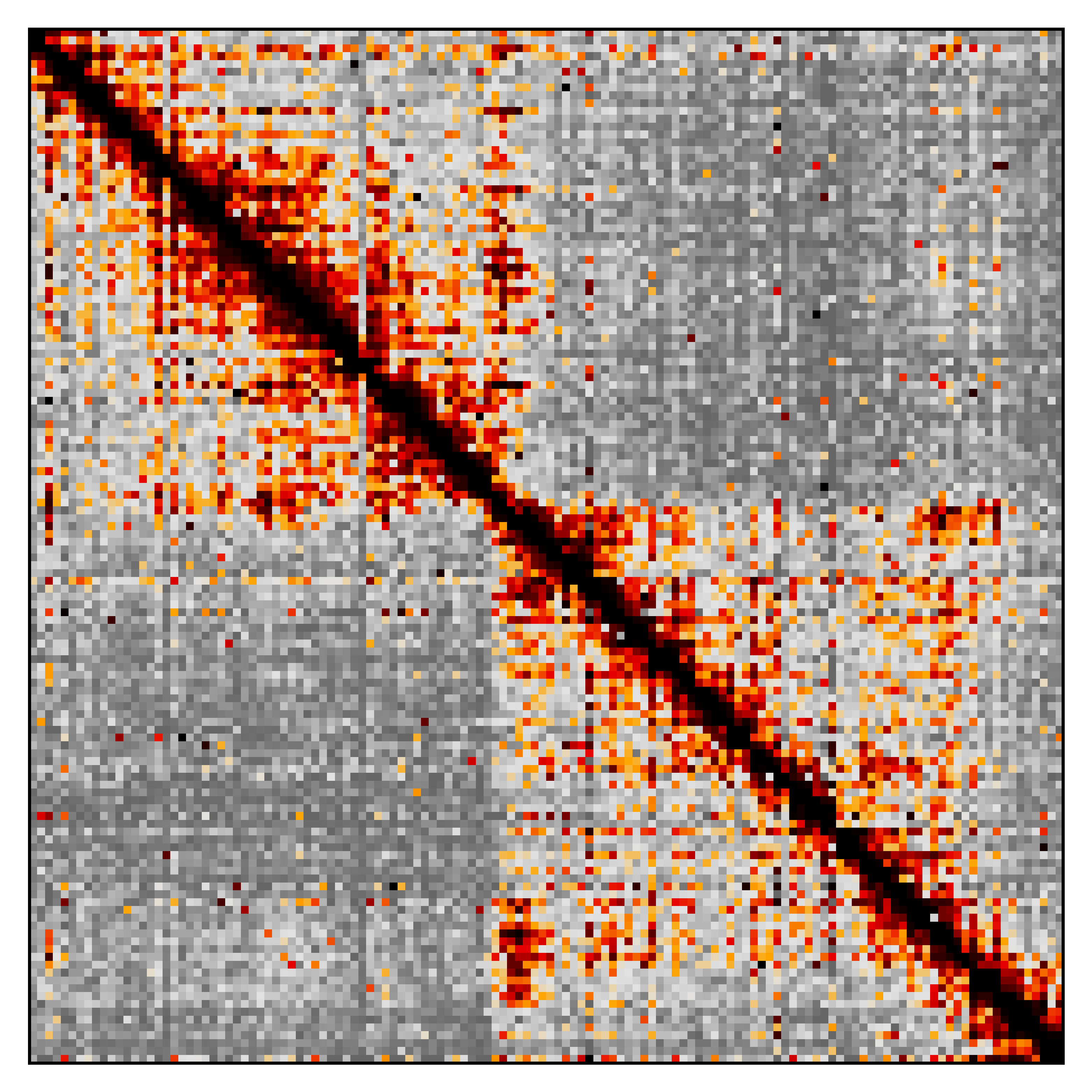
The lib5c plot heatmap subcommand is a lot like the lib5c kr subcommand. In fact, most lib5c subcommands work in almost exactly the same way, so learning to use one can help you understand the others.

Specifying a primerfile/binfile with -p/--primerfile

Almost every lib5c subcommand that takes countsfiles as its input also requires a primerfile or a bedfile that it uses to make sure the countsfiles get parsed correctly. This is accomplished with the -p flag. We didn’t have to use the -p flag in the lib5c kr example above because the primerfile we wanted to use was already in the same directory as the countsfiles, so lib5c was able to find it automatically. In general though, we might be trying to process countsfiles that are separated (directory-wise) from the primerfile that describes their genomic loci, in which case we would have to use the -p flag as shown above.

Multiple output files (one per region)

Some lib5c subcommands generate multiple output files (typically one per region). To create an output file for only one region, use the --region (shorter form -r) as shown above. Alternatively, if we want to generate output for all regions, we can skip the -r/--region flag and include a %r in the outfile instead, which will be replaced with the region name. Combining this with the “multiple input files” idea from above, we can write something like

!lib5c plot heatmap -p trimmed/primers_trimmed.bed 'kr/*.counts' kr/%s_%r.png

lib5c plot heatmap  --primerfile 'trimmed/primers_trimmed.bed' --level 'auto' kr/pNPC_Rep1.counts 'kr/pNPC_Rep1_%r.png' --colormap 'obs' --log_base 'None' --pseudocount '1.0'
loading counts
preparing to plot
plotting
lib5c plot heatmap  --primerfile 'trimmed/primers_trimmed.bed' --level 'auto' kr/pNPC_Rep2.counts 'kr/pNPC_Rep2_%r.png' --colormap 'obs' --log_base 'None' --pseudocount '1.0'
loading counts
preparing to plot
plotting
lib5c plot heatmap  --primerfile 'trimmed/primers_trimmed.bed' --level 'auto' kr/v65_Rep1.counts 'kr/v65_Rep1_%r.png' --colormap 'obs' --log_base 'None' --pseudocount '1.0'
loading counts
preparing to plot
plotting
lib5c plot heatmap  --primerfile 'trimmed/primers_trimmed.bed' --level 'auto' kr/v65_Rep2.counts 'kr/v65_Rep2_%r.png' --colormap 'obs' --log_base 'None' --pseudocount '1.0'
loading counts
preparing to plot
plotting

Binning

Let’s bin our Knight-Ruiz balanced data!

Before we do this, we need to generate some bins to tile our 5C regions. To do this, we run

!lib5c determine-bins -w 4000 trimmed/primers_trimmed.bed bedfiles/4kb_bins.bed

creating directory bedfiles

The -w/--bin_width flag specifies the width of each bin in base pairs, and bedfiles/4kb_bins.bed specifies the name of the newly-created bin bedfile.

Now that we have a bin bedfile describing the bins, we can figure out what the counts values for each bin should be by running

!lib5c bin -w 24000 -p trimmed/primers_trimmed.bed -b bedfiles/4kb_bins.bed kr/pNPC_Rep2.counts binned/pNPC_Rep2.counts

creating directory binned

Notice that the lib5c bin subcommand needs both a primerfile (specified with -p) and a bin bedfile (specified with -b). It needs the primerfile to parse the input files, but it also needs a bin bedfile to know where the bins should be and to write the output files. The last two arguments are just the input file and the output file, just like in the previous subcommands.

We can plot a heatmap of our binned data by running

!lib5c plot heatmap -p bedfiles/4kb_bins.bed -r Sox2 -R -g mm9 binned/pNPC_Rep2.counts binned/pNPC_Rep2_Sox2.png

loading counts
preparing to plot
plotting

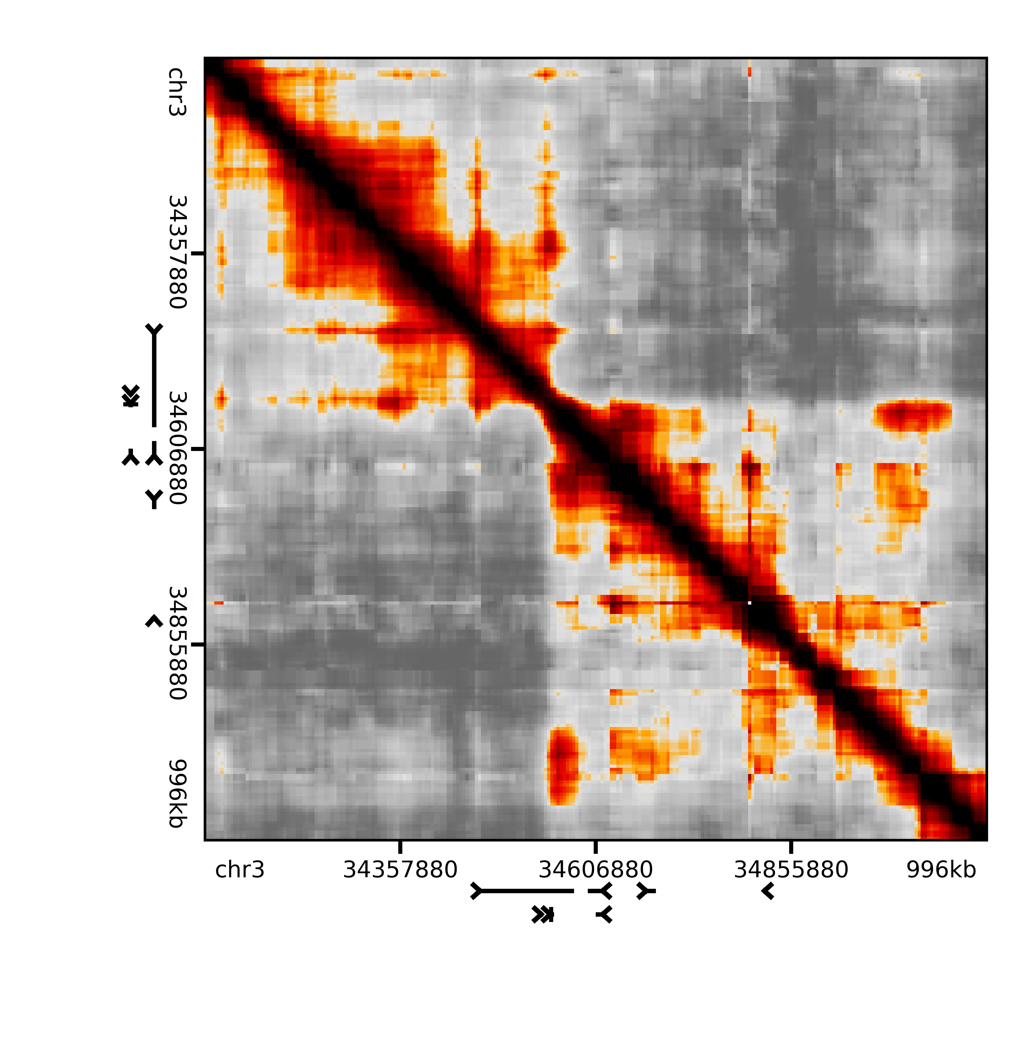
The result should look something like this

Image(filename='binned/pNPC_Rep2_Sox2.png', width=500)

Expected modeling

In order to identify “enriched” interactions in our freshly-binned data, we first need to answer the question: “Enriched with respect to what?” The answer to this question is an expected model, which represents our understanding of what we would expect the interaction frequency between any two bins to be. This expected value depends both on the linear genomic separation between the bins, as well as the effects of local contact domain structure.

We can generate an expected model by running

!lib5c expected -p bedfiles/4kb_bins.bed -RED binned/pNPC_Rep2.counts expected/pNPC_Rep2.counts

loading counts
using polynomial log-log 1-D distance model
using polynomial log-log 1-D distance model
applying donut correction
applying donut correction
creating directory expected

Note that for consistency, the flag used to specify the bin bedfile bedfiles/4kb_bins.bed is still -p. Most lib5c subcommands work on both fragment-level and bin-level data, with essentially no changes to the parameters.

We are using the -R/--regression, -E/--exclude_near_diagonal and -D/--donut_correction flags to indicate that we want to start with a regional expected model fitted with a simple log-log regression which ignores points too close to the diagonal, and then apply donut correction to account for local variations in contact domain structure.

Variance modeling

Armed with an expected model, we can now readily identify which pairs of bins interact more frequently than expected. However, what we really want to know is which pairs of bins interact significantly more frequently than expected. In order to understand the extent of insignificant, noise-driven variations at each point, we need to construct a variance model - a statistical variance estimate for each pair of bins.

We can generate a variance model by running

!lib5c variance -p bedfiles/4kb_bins.bed binned/pNPC_Rep2.counts expected/pNPC_Rep2.counts variance/pNPC_Rep2.counts

loading counts
writing variance
creating directory variance

By default, this will fit a log-normal deviation-based distance-variance relationship to the observed data.

P-value calling

Finally, we will call p-values for the interactions in our dataset

!lib5c pvalues -p bedfiles/4kb_bins.bed binned/pNPC_Rep2.counts expected/pNPC_Rep2.counts variance/pNPC_Rep2.counts -L norm pvalues/pNPC_Rep2.counts

loading counts
calling pvalues
writing p-values
creating directory pvalues

Calling p-values simply parametrizes a distribution of a specified family (here we chose -L norm for the lognormal distribution) with mean value taken from the expected model and variance taken from the variance model, and then calls a right-tail p-value for the observed value in the binned data.

P-value heatmaps

To visualize p-values, we can use the lib5c plot heatmap subcommand as above, but we need to invoke it like

!lib5c plot heatmap -p bedfiles/4kb_bins.bed -r Sox2 -PR -g mm9 pvalues/pNPC_Rep2.counts pvalues/pNPC_Rep2_Sox2.png

loading counts
preparing to plot
plotting

Here we are using the -P/--pvalue flag to indicate that we are trying to visualize p-values, the -R/--rulers flag to indicate that we want to add genomic coordinate rulers to the heatmap, and the -g/--genes flag to indicate that we want to add gene tracks from the mm9 reference genome.

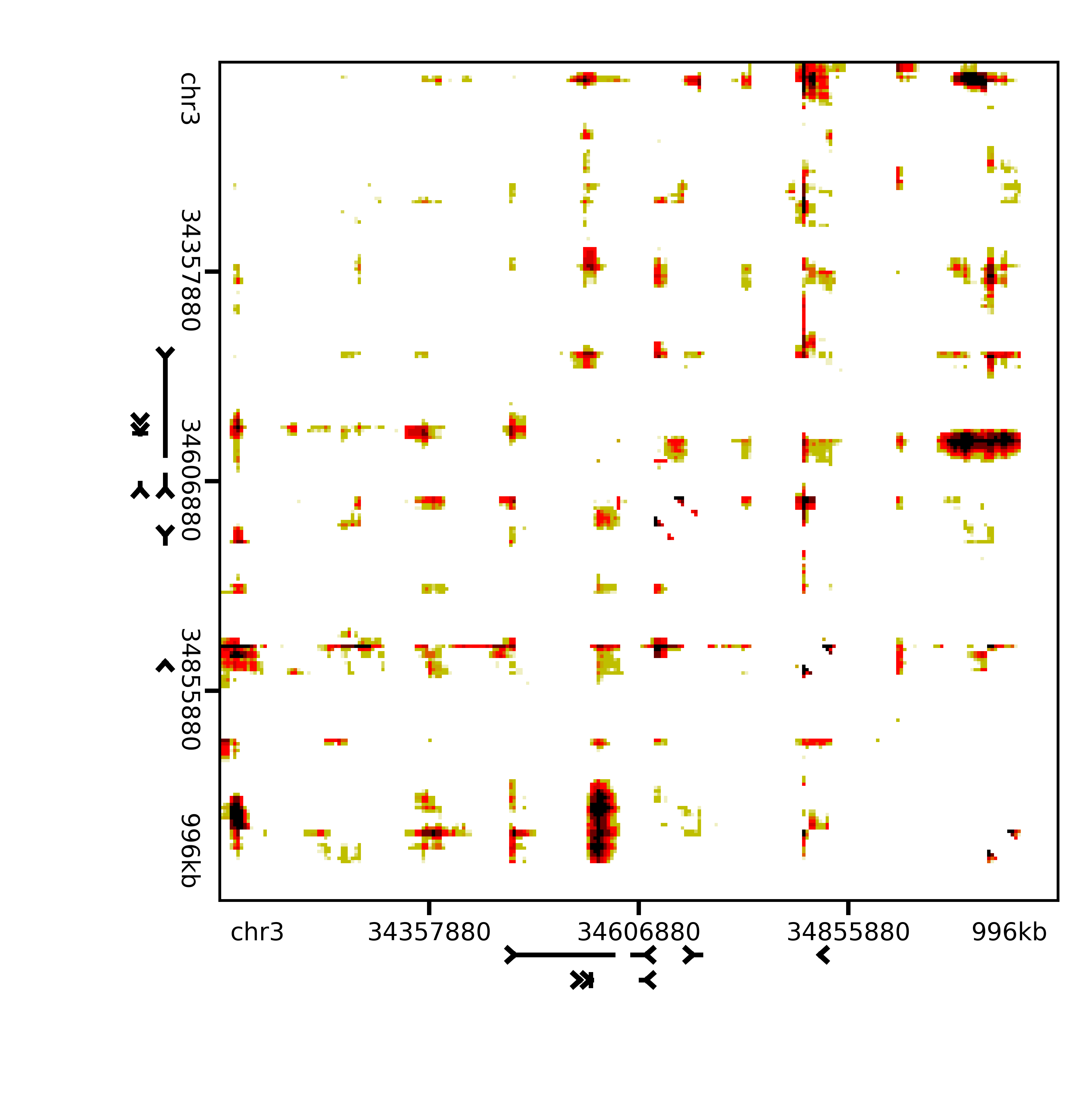
The results should look something like this:

Image(filename='pvalues/pNPC_Rep2_Sox2.png', width=500)

Next steps

Go ahead and explore the other lib5c subcommands! Remember that you can list all the subcommands and get detailed help for a particular subcommand with the -h/--help flag.