Scripting tutorial
This tutorial will walk you through how you might leverage the functions
exposed in lib5c to write your own analysis scripts.
Follow along in Google colab
You can run and modify the cells in this notebook tutorial live using Google colaboratory by clicking the link below:
![]()
To simply have all the cells run automatically, click
Runtime > Run all in the colab toolbar.
Make sure lib5c is installed
Inside a fresh virtual environment, run
In [ ]:
!pip install lib5c
Requirement already satisfied: lib5c in /mnt/c/Users/thoma/venv-doc/lib/python2.7/site-packages (0.5.3)
Requirement already satisfied: numpy>=1.10.4 in /mnt/c/Users/thoma/venv-doc/lib/python2.7/site-packages (from lib5c) (1.14.2)
Requirement already satisfied: pandas>=0.18.0 in /mnt/c/Users/thoma/venv-doc/lib/python2.7/site-packages (from lib5c) (0.22.0)
Requirement already satisfied: statsmodels>=0.6.1 in /mnt/c/Users/thoma/venv-doc/lib/python2.7/site-packages (from lib5c) (0.8.0)
Requirement already satisfied: dill>=0.2.5 in /mnt/c/Users/thoma/venv-doc/lib/python2.7/site-packages (from lib5c) (0.2.7.1)
Requirement already satisfied: luigi>=2.1.1 in /mnt/c/Users/thoma/venv-doc/lib/python2.7/site-packages (from lib5c) (2.7.3)
Requirement already satisfied: matplotlib>=1.4.3 in /mnt/c/Users/thoma/venv-doc/lib/python2.7/site-packages (from lib5c) (2.2.2)
Requirement already satisfied: python-daemon<2.2.0,>=2.1.1 in /mnt/c/Users/thoma/venv-doc/lib/python2.7/site-packages (from lib5c) (2.1.2)
Requirement already satisfied: powerlaw>=1.4.3 in /mnt/c/Users/thoma/venv-doc/lib/python2.7/site-packages (from lib5c) (1.4.3)
Requirement already satisfied: interlap>=0.2.3 in /mnt/c/Users/thoma/venv-doc/lib/python2.7/site-packages (from lib5c) (0.2.6)
Requirement already satisfied: seaborn>=0.8.0 in /mnt/c/Users/thoma/venv-doc/lib/python2.7/site-packages (from lib5c) (0.8.1)
Requirement already satisfied: decorator>=4.0.10 in /mnt/c/Users/thoma/venv-doc/lib/python2.7/site-packages (from lib5c) (4.2.1)
Requirement already satisfied: scikit-learn>=0.17.1 in /mnt/c/Users/thoma/venv-doc/lib/python2.7/site-packages (from lib5c) (0.19.1)
Requirement already satisfied: scipy>=0.16.1 in /mnt/c/Users/thoma/venv-doc/lib/python2.7/site-packages (from lib5c) (1.0.0)
Requirement already satisfied: python-dateutil in /mnt/c/Users/thoma/venv-doc/lib/python2.7/site-packages (from pandas>=0.18.0->lib5c) (2.7.2)
Requirement already satisfied: pytz>=2011k in /mnt/c/Users/thoma/venv-doc/lib/python2.7/site-packages (from pandas>=0.18.0->lib5c) (2018.3)
Requirement already satisfied: patsy in /mnt/c/Users/thoma/venv-doc/lib/python2.7/site-packages (from statsmodels>=0.6.1->lib5c) (0.5.0)
Requirement already satisfied: tornado<5,>=4.0 in /mnt/c/Users/thoma/venv-doc/lib/python2.7/site-packages (from luigi>=2.1.1->lib5c) (4.5.3)
Requirement already satisfied: pyparsing!=2.0.4,!=2.1.2,!=2.1.6,>=2.0.1 in /mnt/c/Users/thoma/venv-doc/lib/python2.7/site-packages (from matplotlib>=1.4.3->lib5c) (2.2.0)
Requirement already satisfied: backports.functools-lru-cache in /mnt/c/Users/thoma/venv-doc/lib/python2.7/site-packages (from matplotlib>=1.4.3->lib5c) (1.5)
Requirement already satisfied: subprocess32 in /mnt/c/Users/thoma/venv-doc/lib/python2.7/site-packages (from matplotlib>=1.4.3->lib5c) (3.5.3)
Requirement already satisfied: six>=1.10 in /mnt/c/Users/thoma/venv-doc/lib/python2.7/site-packages (from matplotlib>=1.4.3->lib5c) (1.11.0)
Requirement already satisfied: kiwisolver>=1.0.1 in /mnt/c/Users/thoma/venv-doc/lib/python2.7/site-packages (from matplotlib>=1.4.3->lib5c) (1.0.1)
Requirement already satisfied: cycler>=0.10 in /mnt/c/Users/thoma/venv-doc/lib/python2.7/site-packages (from matplotlib>=1.4.3->lib5c) (0.10.0)
Requirement already satisfied: setuptools in /mnt/c/Users/thoma/venv-doc/lib/python2.7/site-packages (from python-daemon<2.2.0,>=2.1.1->lib5c) (40.4.3)
Requirement already satisfied: docutils in /mnt/c/Users/thoma/venv-doc/lib/python2.7/site-packages (from python-daemon<2.2.0,>=2.1.1->lib5c) (0.14)
Requirement already satisfied: lockfile>=0.10 in /mnt/c/Users/thoma/venv-doc/lib/python2.7/site-packages (from python-daemon<2.2.0,>=2.1.1->lib5c) (0.12.2)
Requirement already satisfied: backports-abc>=0.4 in /mnt/c/Users/thoma/venv-doc/lib/python2.7/site-packages (from tornado<5,>=4.0->luigi>=2.1.1->lib5c) (0.5)
Requirement already satisfied: certifi in /mnt/c/Users/thoma/venv-doc/lib/python2.7/site-packages (from tornado<5,>=4.0->luigi>=2.1.1->lib5c) (2018.1.18)
Requirement already satisfied: singledispatch in /mnt/c/Users/thoma/venv-doc/lib/python2.7/site-packages (from tornado<5,>=4.0->luigi>=2.1.1->lib5c) (3.4.0.3)
Make a directory and get data
If you haven’t completed the pipeline tutorial yet, make a directory for the tutorial:
$ mkdir lib5c-tutorial
$ cd lib5c-tutorial
and prepare the example data in lib5c-tutorial/input as shown in the
pipeline tutorial.
In [2]:
!mkdir input
!wget -qO- 'http://www.ncbi.nlm.nih.gov/geo/download/?acc=GSE68582&format=file&file=GSE68582%5FBED%5FES%2DNPC%2DiPS%2DLOCI%5Fmm9%2Ebed%2Egz' | gunzip -c > input/BED_ES-NPC-iPS-LOCI_mm9.bed
!wget -qO- 'http://www.ncbi.nlm.nih.gov/geo/download/?acc=GSM1974095&format=file&file=GSM1974095%5Fv65%5FRep1%2Ecounts%2Etxt%2Egz' | gunzip -c > input/v65_Rep1.counts
!wget -qO- 'http://www.ncbi.nlm.nih.gov/geo/download/?acc=GSM1974096&format=file&file=GSM1974096%5Fv65%5FRep2%2Ecounts%2Etxt%2Egz' | gunzip -c > input/v65_Rep2.counts
!wget -qO- 'http://www.ncbi.nlm.nih.gov/geo/download/?acc=GSM1974099&format=file&file=GSM1974099%5FpNPC%5FRep1%2Ecounts%2Etxt%2Egz' | gunzip -c > input/pNPC_Rep1.counts
!wget -qO- 'http://www.ncbi.nlm.nih.gov/geo/download/?acc=GSM1974100&format=file&file=GSM1974100%5FpNPC%5FRep2%2Ecounts%2Etxt%2Egz' | gunzip -c > input/pNPC_Rep2.counts
!sed -i '/Sox2\|Klf4/!d' input/BED_ES-NPC-iPS-LOCI_mm9.bed
mkdir: cannot create directory ‘input’: File exists
Note for Docker image users
If you are using lib5c from the Docker image, run
$ docker run -it -v <full path to lib5c-tutorial>:/lib5c-tutorial creminslab/lib5c:latest
root@<container_id>:/# cd /lib5c-tutorial
and continue running all tutorial commands in this shell.
Start an interactive session
To quickly get used to calling the functions in lib5c, we recommend
trying out the following code snippets in a Python interactive session,
which we can start by running
$ python
from inside the lib5c-tutorial directory.
If you’re following along in the IPython notebook, you’re already in a Python interactive session and don’t need to do anything.
Of course, you’re welcome to write scripts and execute them with commands like
$ python myscript.py
Basic parsing and writing
Parsing
In order to perform any operation on our data, we need to load the data into memory first. Many functions for parsing various types of data are exposed in the lib5c.parsers subpackage. For this tutorial, we will use the following four parsers:
- lib5c.parsers.primers.load_primermap() for parsing bedfiles which describe the genomic coordinates and context of the rows and columns of a contact matrix into primermaps
- lib5c.parsers.counts.load_counts() for parsing countsfiles into counts dicts (dictionaries of contact matrices)
For more detail on these data structures and file types, see the section on Core data structures and file types.
Writing
After we apply some operations to our data, we often want to save our results by writing data back to the disk. Many functions for writing various types of data to the disk are exposed in the lib5c.writers subpackage. The writing functions that parallel the parsers listed above are:
- lib5c.writers.primers.write_primermap() for writing primer and bin bedfiles
- lib5c.writers.counts.write_counts() for writing countsfiles
Normalization
For our first script, we will apply the Knight-Ruiz algorithm to some of our data.
First, we need to load information about the primers used in the 5C experiment. We need to do this before we parse the fragment-level raw countsfiles to make sure we parse them correctly.
In [3]:
from lib5c.parsers.primers import load_primermap
primermap = load_primermap('input/BED_ES-NPC-iPS-LOCI_mm9.bed')
Now we can parse a countsfile into a counts dict.
In [4]:
from lib5c.parsers.counts import load_counts
counts = load_counts('input/v65_Rep1.counts', primermap)
Notice that we had to pass the primermap as an argument to
lib5c.parsers.counts.load_counts().
Before balancing the counts matrices, we should remove some low-quality primers which may impair the matrix balancing process. We actually want to do this on the basis of primer quality across all the replicates. To do this, we can leverage the exposed functions lib5c.algorithms.trimming.trim_primers() and lib5c.algorithms.trimming.trim_counts() to do
In [5]:
from lib5c.algorithms.trimming import trim_primers, trim_counts
reps = ['v65_Rep1', 'v65_Rep2', 'pNPC_Rep1', 'pNPC_Rep2']
counts_superdict = {rep: load_counts('input/%s.counts' % rep, primermap) for rep in reps}
trimmed_primermap, trimmed_indices = trim_primers(primermap, counts_superdict)
trimmed_counts = trim_counts(counts, trimmed_indices)
For more details, consult the section on Trimming.
Now we can balance the counts matrices. To do this, we will use the
function
lib5c.algorithms.knight_ruiz.kr_balance_matrix().
Most algorithms in lib5c live in the
lib5c.algorithms subpackage and expose some
sort of convenience function. To learn more about the various
convenience functions and APIs exposed in lib5c, consult the section
on API specification and conceptual documentation
Go ahead and import this function with
In [6]:
from lib5c.algorithms.knight_ruiz import kr_balance_matrix
To balance the matrix for the Sox2 region, we can try
In [7]:
kr_counts_Sox2, bias_Sox2, _ = kr_balance_matrix(trimmed_counts['Sox2'])
To check how balanced the result is, we can immediately check
In [8]:
import numpy as np
row_sums = np.nansum(kr_counts_Sox2, axis=0)
row_sums[:10]
Out[8]:
array([14291.21482377, 14291.21505217, 14291.2145544 , 14291.21481292,
       14291.21477069, 14291.21475874, 14291.21456383, 14291.21706808,
       14291.21470187, 14291.21831915])
In [9]:
np.max(np.abs(np.mean(row_sums) - row_sums))
Out[9]:
0.004428315922268666
For more details on matrix balancing, consult the section on Bias mitigation.
Analyzing multiple regions in parallel
Most of the convenience functions exposed in lib5c are decorated
with a special decorator, @parallelize_regions, that parallelizes
their operation across the regions of a counts dict. For more
information on this decorator, see the section on Parallelization
across regions.
For the purposes of this tutorial, all this means is that we can try something like
In [10]:
kr_counts, bias_vectors, _ = kr_balance_matrix(trimmed_counts)
to balance all the matrices in the counts dict. To check how balanced one of the matrices is, we can check
In [11]:
row_sums = np.nansum(kr_counts['Klf4'], axis=0)
row_sums[:10]
Out[11]:
array([10655.10469556, 10655.10482373, 10655.10468786, 10655.10479662,
       10655.10478073, 10655.10475555, 10655.10485518, 10655.1048237 ,
       10655.10477974, 10655.10498231])
In [12]:
np.max(np.abs(np.mean(row_sums) - row_sums))
Out[12]:
0.001775397115125088
Notice that the returned object kr_counts is a dict indexed by
region name, just like the input argument counts.
Finally, we can save the results of our processing with something like
In [13]:
from lib5c.writers.counts import write_counts
write_counts(kr_counts, 'scripting/v65_Rep1_kr.counts', trimmed_primermap)
creating directory scripting
We should save our trimmed primer set as well so that we don’t have to redo the trimming step every time we load this data.
In [14]:
from lib5c.writers.primers import write_primermap
write_primermap(trimmed_primermap, 'scripting/primers_trimmed.bed')
Binning
If you closed out of the previous session, you’ll need to read back in the data we were working with. Try
In [15]:
from lib5c.parsers.primers import load_primermap
primermap = load_primermap('scripting/primers_trimmed.bed')
from lib5c.parsers.counts import load_counts
kr_counts = load_counts('scripting/v65_Rep1_kr.counts', primermap)
Ultimately, we will want to use the exposed convenience function
lib5c.algorithms.filtering.fragment_bin_filtering.fragment_bin_filter().
According to the docstring, it looks like we will need a pixelmap
and a filter_function in addition to our counts dict.
The pixelmap represents where our bins should be. To generate one,
we will use the exposed convenience function
lib5c.algorithms.determine_bins.determine_regional_bins(),
which can be used to do something like
In [16]:
from lib5c.algorithms.determine_bins import determine_regional_bins
pixelmap = determine_regional_bins(primermap, 4000, region_name={region: region for region in primermap.keys()})
The filter_function represents the filtering function to be passed
over the counts matrices in order to determine the value in each bin. To
construct one, we can use the exposed convenience function
lib5c.algorithms.filtering.filter_functions.make_filter_function(),
which can be used to do something like
In [17]:
from lib5c.algorithms.filtering.filter_functions import make_filter_function
filter_function = make_filter_function()
Finally, we can bin our counts with a 20 kb window radius by trying
In [18]:
from lib5c.algorithms.filtering.fragment_bin_filtering import fragment_bin_filter
binned_counts = fragment_bin_filter(kr_counts, filter_function, pixelmap, primermap, 20000)
To save these counts to disk, we can run
In [19]:
from lib5c.writers.counts import write_counts
write_counts(binned_counts, 'scripting/v65_Rep1_binned.counts', pixelmap)
We can also write the pixelmap we created to the disk as a bin bedfile by trying
In [20]:
from lib5c.writers.primers import write_primermap
write_primermap(pixelmap, 'scripting/4kb_bins.bed')
For more information about the filtering/binning/smoothing API, see the section on Binning and smoothing.
Plotting heatmaps
If you closed out of the previous session, you’ll need to read back in the data we were working with. Try
In [21]:
from lib5c.parsers.primers import load_primermap
pixelmap = load_primermap('scripting/4kb_bins.bed')
from lib5c.parsers.counts import load_counts
binned_counts = load_counts('scripting/v65_Rep1_binned.counts', pixelmap)
To visualize our binned matrices, we can use the exposed function lib5c.plotters.heatmap.plot_heatmap().
Before we start, it’s a good idea to transform the counts values to a log scale for easier visualization
In [22]:
import numpy as np
logged_counts = {region: np.log(binned_counts[region] + 1) for region in binned_counts.keys()}
First, we need to import the plotting function with
In [23]:
from lib5c.plotters.heatmap import plot_heatmap
We can draw the heatmap for just one region with
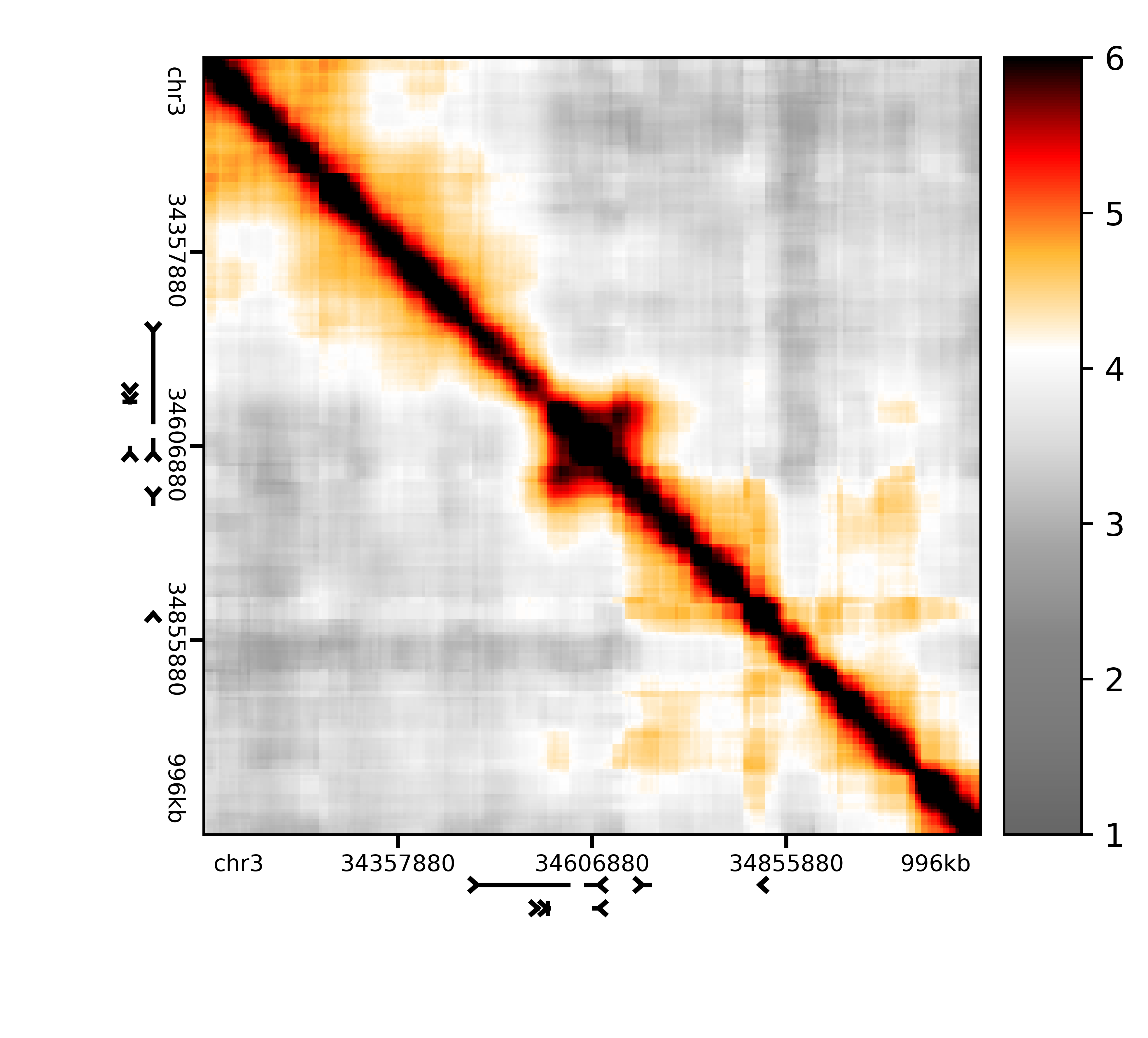
In [24]:
%matplotlib notebook
plot_heatmap(logged_counts['Sox2'], grange_x=pixelmap['Sox2'], rulers=True, genes='mm9', colorscale=(1.0, 6.0), colorbar=True, outfile='scripting/v65_Rep1_binned_Sox2.png')
Out[24]:
(<matplotlib.axes._subplots.AxesSubplot at 0x7f4dacce8650>,
 <lib5c.plotters.extendable.extendable_heatmap.ExtendableHeatmap at 0x7f4db3507b50>)
The resulting image should look something like this:
In [25]:
from IPython.display import Image
Image(filename='scripting/v65_Rep1_binned_Sox2.png', width=500)
Out[25]:
Because
plot_heatmap()
is parallelized with the @parallelize_regions decorator, we can draw
the heatmaps for all regions at once by simply calling
In [26]:
%matplotlib notebook
outfile_names = {region: 'scripting/v65_Rep1_binned_%s.png' % region for region in binned_counts.keys()}
plot_heatmap(logged_counts, grange_x=pixelmap, rulers=True, genes='mm9', colorscale=(1.0, 6.0), colorbar=True, outfile=outfile_names)
encountered exception, falling back to series operation
Out[26]:
<generator object <genexpr> at 0x7f4da9966e10>
where we precompute a dict of output filenames (parallel to
counts_binned) to describe where each region’s heatmap will get
drawn (since each region will be drawn to a separate heatmap). In this
way, any argument to a parallelized function can be replaced by a dict
whose keys match the keys of the first positional argument (which is
usually a counts dict).
You can show the plot directly inline in a notebook environment by
skipping the outfile kwarg:
In [27]:
%matplotlib inline
plot_heatmap(logged_counts['Sox2'], grange_x=pixelmap['Sox2'], rulers=True, genes='mm9', colorscale=(1.0, 6.0), colorbar=True)
Out[27]:
(<matplotlib.axes._axes.Axes at 0x7f4d9512c110>,
 <lib5c.plotters.extendable.extendable_heatmap.ExtendableHeatmap at 0x7f4db239da90>)
Expected modeling
The exposed convenience function for making an expected model is lib5c.algorithms.expected.make_expected_matrix().
To construct an expected model for each region using a simple power law relationship and apply donut correction in the same step, we can try
In [28]:
from lib5c.algorithms.expected import make_expected_matrix
exp_counts, dist_exp, _ = make_expected_matrix(binned_counts, regression=True, exclude_near_diagonal=True, donut=True)
using polynomial log-log 1-D distance model
using polynomial log-log 1-D distance model
applying donut correction
applying donut correction
The first returned value, counts_exp, is simply a dict of the
expected matrices representing the model. The second returned value,
dist_exp, is a representation of the simple one-dimensional expected
model.
We can visualize the one-dimensional expected model using lib5c.plotters.expected.plot_bin_expected().
In [29]:
%matplotlib notebook
from lib5c.plotters.expected import plot_bin_expected
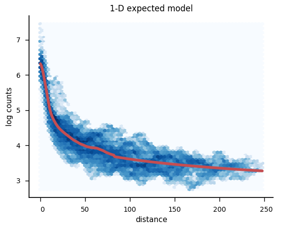
plot_bin_expected(binned_counts['Sox2'], dist_exp['Sox2'], outfile='scripting/v65_Rep1_expected_model_Sox2.png', hexbin=True, semilog=True, xlabel='distance')
Out[29]:
<matplotlib.axes._subplots.AxesSubplot at 0x7f4dad328c50>
or for all regions at once,
In [30]:
%matplotlib notebook
from lib5c.plotters.expected import plot_bin_expected
outfile_names = {region: 'scripting/v65_Rep1_expected_model_%s.png' % region for region in binned_counts.keys()}
plot_bin_expected(binned_counts, dist_exp, outfile=outfile_names, hexbin=True, semilog=True, xlabel='distance')
Out[30]:
{'Klf4': <matplotlib.axes._subplots.AxesSubplot at 0x7f4dad1ee850>,
 'Sox2': <matplotlib.axes._subplots.AxesSubplot at 0x7f4da07fae90>}
The kwargs hexbin, semilog, and ylabel tweak the visual
appearance of the resulting plot.
The resulting images should look something like this:
In [31]:
Image(filename='scripting/v65_Rep1_expected_model_Sox2.png', width=500)
Out[31]:
To learn more, consult the section on Expected modeling.
Variance modeling
The exposed convenience functions for variance modeling is lib5c.algorithms.variance.estimate_variance().
We can get variance estimates from a log-normal, deviation-based distance-variance relationship model by trying
In [32]:
from lib5c.algorithms.variance import estimate_variance
var_counts = estimate_variance(binned_counts, exp_counts)
To learn more, consult the section on Variance modeling.
P-value calling
The exposed convenience function for calling p-values using distributions parametrized according to the expected and variance models is lib5c.util.distributions.call_pvalues().
To simply call the p-values using a log-normal distribution, we can try
In [33]:
from lib5c.util.distributions import call_pvalues
from lib5c.util.counts import parallel_log_counts
pvalues = call_pvalues(parallel_log_counts(binned_counts), exp_counts, var_counts, 'norm', log=True)
Where we are logging the observed counts and comparing them to a normal distribution.
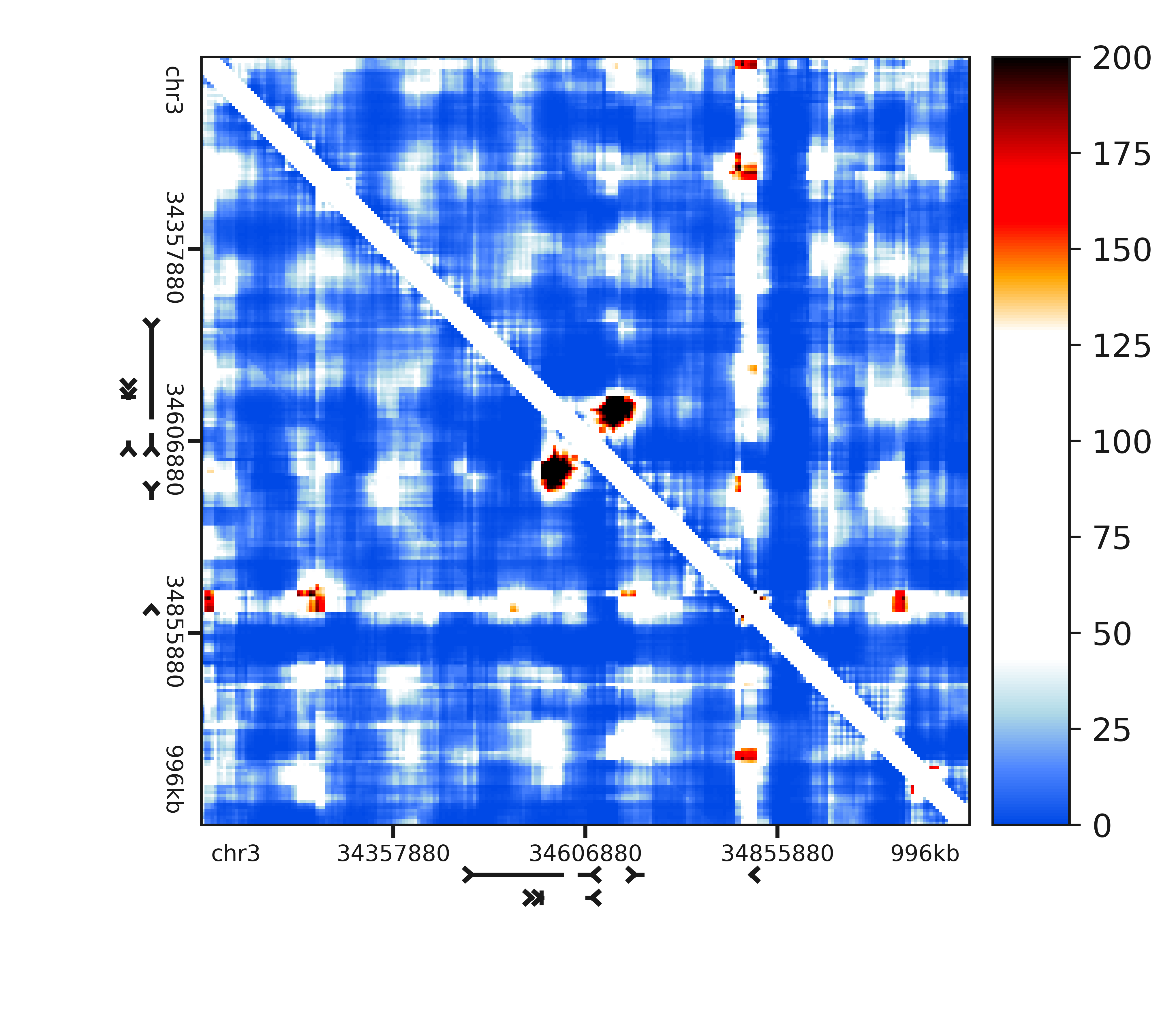
We can visualize these called p-values as interaction scores
(-10*log2(pvalue)) on heatmaps by calling
In [34]:
%matplotlib notebook
from lib5c.plotters.heatmap import plot_heatmap
from lib5c.util.counts import convert_pvalues_to_interaction_scores
outfile_names = {region: 'scripting/v65_Rep1_is_%s.png' % region for region in pvalues.keys()}
interaction_scores = convert_pvalues_to_interaction_scores(pvalues)
plot_heatmap(interaction_scores, grange_x=pixelmap, rulers=True, genes='mm9', colorscale=(0, 200), colorbar=True, colormap='is', outfile=outfile_names)
encountered exception, falling back to series operation
Out[34]:
<generator object <genexpr> at 0x7f4d685e8cd0>
and write them to the disk by calling
In [35]:
from lib5c.writers.counts import write_counts
write_counts(pvalues, 'scripting/v65_Rep1_pvalues.counts', pixelmap)
The resulting images should look something like this
In [36]:
Image(filename='scripting/v65_Rep1_is_Sox2.png', width=500)
Out[36]:
For more information on the distribution fitting and p-value calling API, see the section on Distribution fitting.
Next steps
This tutorial shows only a few of the functions exposed in the lib5c
API. You can read more about what you can do with lib5c in the
section on API specification and conceptual
documentation.